
Leaflet in R
Some time ago we showed you how to display the results of your analyses on maps using ggmap. Today we’ll show you how to use the leaflet package in R to create interactive maps. To do this, we need the raster and sf libraries to load and process the input layers:
|
1 2 3 |
library(leaflet) library(raster) library(sf) |
For our exercise, we will use the vector layers we used before: railways and roads. Let’s load them:
|
1 2 |
railways <- st_read("d:/railways.shp") roads <- st_read("d:/road.shp") |
Let’s find the railway crossings:
|
1 |
railway_crossings <- st_intersection(railways,roads) |
Let’s load the raster. We will use the DEM for the Mazovia region:
|
1 |
dem <- raster("d:/mazovia_dem.tif") |
The loaded raster does not have a coordinate system associated with it yet. Let’s correct that:
|
1 |
projection(dem) = CRS("+init=EPSG:2180") |
We will clip the NMT to the extent of the road layer:
|
1 |
dem <- crop(dem,roads) |
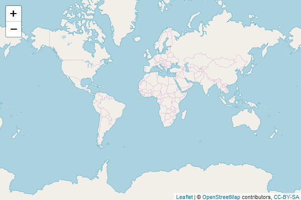
Let’s open the map base with Leaflet and add implicit OSM map base tiles:
|
1 |
m <- leaflet() %>% addTiles() |
Let’s display the map:
|
1 |
m |
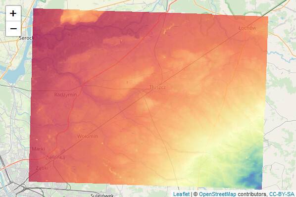
Let’s add a raster DEM to the map, with a transparency of 0.8 function addRasterImage:
|
1 2 |
m %>% addRasterImage(dem, opacity = 0.8, group = "DEM") |
Let’s add a layer with roads (blue) and railways (red) using addPolylines. For vector layers, it is necessary to transform to a geographic layout with st_transform:
|
1 2 3 4 |
m %>% addRasterImage(dem, opacity = 0.8, group = "DEM") %>% addPolylines(data = st_transform(railways,4326), group = "Railways") %>% addPolylines(data = st_transform(roads,4326), color = "red", group = "Roads") |

Previously, we intersected the two loaded layers, creating a point layer with intersections. Let’s add them to our map with addCircleMakers:
|
1 2 3 4 5 |
m %>% addRasterImage(dem, opacity = 0.8, group = "DEM") %>% addPolylines(data = st_transform(railways,4326), group = "Railways") %>% addPolylines(data = st_transform(roads,4326), color = "red", group = "Roads") %>% addCircleMarkers(data = st_transform(railway_crossing,4326), color = "green", group = "Railway crossings") |
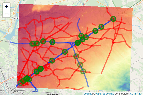
Our map now contains all the layers. The map is interactive – we can move around freely in it.
Czy zwróciliście uwagę że dla każdej funkcji dodającej warstwę zdefiniowaliśmy atrybut group. Wartości tego atrybutu wykorzystamy w ostatnim kroku dodając do mapy listę warstw. Podzielimy warstwy na te wyświetlane niezależnie (baseGroups) i te które mogą się nakładać (overlayGroups).
Did you notice that we defined a group attribute for each function to add a layer. We will use the values of this attribute in the last step when adding a list of layers to the map. We will divide the layers into those that are displayed independently (baseGroups) and those that can overlap (overlayGroups).
|
1 2 3 4 5 6 |
m %>% addRasterImage(dem, opacity = 0.8, group = "DEM") %>% addPolylines(data = st_transform(railways,4326), group = "Railways") %>% addPolylines(data = st_transform(roads,4326), color = "red", group = "Roads") %>% addCircleMarkers(data = st_transform(railway_crossings,4326), color = "green", group = "Railway crossings") %>% addLayersControl(baseGroups = c("Railways","Roads"), overlayGroups = c("Railway crossings","DEM")) |
In the end, the map looks and works like this:
This post was just to give you an idea of what the leaflet package can do. It has many more features not mentioned today that you will have to discover for yourself. You can learn more about the features of the raster and sf libraries in our course GIS in R.
